Day 2 - HIV exercises
Table of Contents
While we were provided materials for the toy examples in day one, I have to download the HIV data for day two myself. At least we have the sources in the materials, so it shouldn’t be a problem, and I would like to do this before starting with our own bacterial data. I also have an RMarkdown protocol from my group for this day which I will partly follow.
Getting started
Let’s see where the example data is…
Reference sequences for the five HIV strains used are directly located in the referenced GitHub repo, and raw reads (Illumina, PacBio, and 454) of a mix of all five strains can theoretically be downloaded from SRA. In practice, the links given in the repo do not work, but the data still exists at NCBI.
cd /data3/genome_graphs/CPANG/static/playground
mkdir day2
cd day2
fastq-dump SRR961514
2019-10-18T08:57:38 fastq-dump.2.3.5 err: error unexpected while resolving tree within virtual file system module - failed to resolve accession 'SRR961514' - Obsolete software. See https://github.com/ncbi/sra-tools/wiki/Obsolete-software ( 406 )

Redirected!!!

2019-10-18T08:57:39 fastq-dump.2.3.5 err: name incorrect while evaluating path within network system module - Scheme is 'https'
2019-10-18T08:57:39 fastq-dump.2.3.5 err: item not found while constructing within virtual database module - the path 'SRR961514' cannot be opened as database or table
spo12@CPI-SL64001:/data3/genome_graphs/CPANG/playground/day2$ fastq-dump SRX342702
2019-10-18T08:58:56 fastq-dump.2.3.5 err: error unexpected while resolving tree within virtual file system module - failed to resolve accession 'SRX342702' - Obsolete software. See https://github.com/ncbi/sra-tools/wiki/Obsolete-software ( 406 )

Redirected!!!

2019-10-18T08:58:56 fastq-dump.2.3.5 err: name incorrect while evaluating path within network system module - Scheme is 'https'
2019-10-18T08:58:56 fastq-dump.2.3.5 err: item not found while constructing within virtual database module - the path 'SRX342702' cannot be opened as database or table
Sadly, we have an old version of the SRA Toolkit installed, so I would have to clean that up before I can download the data, or I can just do it manually…
mkdir reads
cd reads
fastq-dump SRR961669.2
fastq-dump SRR961514.1
cd ..
Not all of the files listed online could be downloaded by simply clicking on them, but I have a set of PacBio reads (SRR961669) and a set of Illumina reads (SRR961514) now, that should be enough to play around with.
Previous aims
During the course, my group’s aims were to compare different variant graph construction methods as well as finding variation in viral genes. I’m not going to retrace all the steps we took (like the de novo assembly of PacBio reads), but at least the parts I can do without installing additional software I might not need later on.
AIM 1 - Construction methods for genome graphs
For this part, we used HIV-1 (which was also provided in the course) together with the five reference sequences to create a genome graph for HIV. The complete HIV-1 genome can be found at NCBI.
vg msga with a single genome graph as base
First, we created and indexed a genome graph based solely on HIV-1.
wget ftp://ftp.ncbi.nlm.nih.gov/genomes/all/GCF/000/864/765/GCF_000864765.1_ViralProj15476/GCF_000864765.1_ViralProj15476_genomic.fna.gz
gunzip GCF_000864765.1_ViralProj15476_genomic.fna.gz
vg construct -r GCF_000864765.1_ViralProj15476_genomic.fna > hiv.vg
vg index -x hiv.xg hiv.vg -g hiv.gcsa
vg msga -f REF.fasta -g hiv.vg > hiv_6genomes.vg
Then we used vg msga to create a multiple sequence alignment of the five reference sequences together with the graph, writing everything in the form of a new variant graph.
This was already too big for the standard DOT format, so we visualised it in Bandage instead:
vg view hiv_6genomes.vg > hiv_6genomes.gfa

Variant graph in Bandage
I’d also like to try the Inkscape method suggested in the course instructions as well:
vg index -x hiv_6genomes.xg hiv_6genomes.vg
vg viz -x hiv_6genomes.xg -o hiv_6genomes.svg
This kind of visualisation is much nicer, since you can see the paths of the genomes through the graph:
Variant graph with vg viz and Inkscape - start
Variant graph with vg viz and Inkscape - random region
minimap2 with seqwish and odgi
Another way to generate a genome graph from the six given reference genomes is creating a multiple sequence alignment (MSA) with minimap2 and then using Erik’s tool seqwish to create a graph from that. This graph can be visualised and manipulated with odgi, another tool from the vg team.
Installing minimap2, seqwish, and odgi
To be able to that, I first have to install those tools…
cd ../../../
git clone https://github.com/lh3/minimap2
cd minimap2 && make
git clone https://github.com/ekg/seqwish
cd seqwish
cmake -H. -Bbuild && cmake --build build -- -j3
git clone https://github.com/vgteam/odgi
cd odgi
cmake -H. -Bbuild && cmake --build build -- -j 3
cd /usr/bin/
sudo ln -s /data3/genome_graphs/minimap2/minimap2
sudo ln -s /data3/genome_graphs/seqwish/bin/seqwish
cd /data3/genome_graphs/
Minimap2 and seqwish were really easy to install, but odgi ended in an error message:
Scanning dependencies of target odgi_pybind11
[100%] Building CXX object CMakeFiles/odgi_pybind11.dir/src/pythonmodule.cpp.o
In file included from /data3/genome_graphs/odgi/deps/pybind11/include/pybind11/pytypes.h:12:0,
                 from /data3/genome_graphs/odgi/deps/pybind11/include/pybind11/cast.h:13,
                 from /data3/genome_graphs/odgi/deps/pybind11/include/pybind11/attr.h:13,
                 from /data3/genome_graphs/odgi/deps/pybind11/include/pybind11/pybind11.h:44,
                 from /data3/genome_graphs/odgi/src/pythonmodule.cpp:6:
/data3/genome_graphs/odgi/deps/pybind11/include/pybind11/detail/common.h:112:20: fatal error: Python.h: No such file or directory
compilation terminated.
CMakeFiles/odgi_pybind11.dir/build.make:62: recipe for target 'CMakeFiles/odgi_pybind11.dir/src/pythonmodule.cpp.o' failed
make[2]: *** [CMakeFiles/odgi_pybind11.dir/src/pythonmodule.cpp.o] Error 1
CMakeFiles/Makefile2:318: recipe for target 'CMakeFiles/odgi_pybind11.dir/all' failed
make[1]: *** [CMakeFiles/odgi_pybind11.dir/all] Error 2
make[1]: *** Waiting for unfinished jobs....
[100%] Built target odgi
Makefile:83: recipe for target 'all' failed
make: *** [all] Error 2
I’ll try building pybind11 “manually”:
cd odig/deps/pybind11/
mkdir build
cd build
cmake ..
CMake Error at tests/CMakeLists.txt:217 (message):
  Running the tests requires pytest.  Please install it manually (try:
  /usr/bin/python3.6 -m pip install pytest)


-- Configuring incomplete, errors occurred!
See also "/data3/genome_graphs/odgi/deps/pybind11/build/CMakeFiles/CMakeOutput.log".
/usr/bin/python3.6 -m pip install pytest
cmake ..
make check -j 4
The cmake call worked now, but make check ended in the same error as before:
Scanning dependencies of target cross_module_gil_utils
[  2%] Building CXX object tests/CMakeFiles/cross_module_gil_utils.dir/cross_module_gil_utils.cpp.o
In file included from /data3/genome_graphs/odgi/deps/pybind11/include/pybind11/pytypes.h:12:0,
                 from /data3/genome_graphs/odgi/deps/pybind11/include/pybind11/cast.h:13,
                 from /data3/genome_graphs/odgi/deps/pybind11/include/pybind11/attr.h:13,
                 from /data3/genome_graphs/odgi/deps/pybind11/include/pybind11/pybind11.h:44,
                 from /data3/genome_graphs/odgi/deps/pybind11/tests/cross_module_gil_utils.cpp:9:
/data3/genome_graphs/odgi/deps/pybind11/include/pybind11/detail/common.h:112:20: fatal error: Python.h: No such file or directory
compilation terminated.
tests/CMakeFiles/cross_module_gil_utils.dir/build.make:62: recipe for target 'tests/CMakeFiles/cross_module_gil_utils.dir/cross_module_gil_utils.cpp.o' failed
make[3]: *** [tests/CMakeFiles/cross_module_gil_utils.dir/cross_module_gil_utils.cpp.o] Error 1
CMakeFiles/Makefile2:197: recipe for target 'tests/CMakeFiles/cross_module_gil_utils.dir/all' failed
make[2]: *** [tests/CMakeFiles/cross_module_gil_utils.dir/all] Error 2
make[2]: *** Waiting for unfinished jobs....
tests/test_cmake_build/CMakeFiles/test_subdirectory_target.dir/build.make:57: recipe for target 'tests/test_cmake_build/CMakeFiles/test_subdirectory_target' failed
make[3]: *** [tests/test_cmake_build/CMakeFiles/test_subdirectory_target] Error 1
CMakeFiles/Makefile2:467: recipe for target 'tests/test_cmake_build/CMakeFiles/test_subdirectory_target.dir/all' failed
make[2]: *** [tests/test_cmake_build/CMakeFiles/test_subdirectory_target.dir/all] Error 2
tests/test_cmake_build/CMakeFiles/test_subdirectory_embed.dir/build.make:57: recipe for target 'tests/test_cmake_build/CMakeFiles/test_subdirectory_embed' failed
make[3]: *** [tests/test_cmake_build/CMakeFiles/test_subdirectory_embed] Error 1
CMakeFiles/Makefile2:300: recipe for target 'tests/test_cmake_build/CMakeFiles/test_subdirectory_embed.dir/all' failed
make[2]: *** [tests/test_cmake_build/CMakeFiles/test_subdirectory_embed.dir/all] Error 2
tests/test_cmake_build/CMakeFiles/test_subdirectory_function.dir/build.make:57: recipe for target 'tests/test_cmake_build/CMakeFiles/test_subdirectory_function' failed
make[3]: *** [tests/test_cmake_build/CMakeFiles/test_subdirectory_function] Error 1
CMakeFiles/Makefile2:327: recipe for target 'tests/test_cmake_build/CMakeFiles/test_subdirectory_function.dir/all' failed
make[2]: *** [tests/test_cmake_build/CMakeFiles/test_subdirectory_function.dir/all] Error 2
CMakeFiles/Makefile2:237: recipe for target 'tests/CMakeFiles/check.dir/rule' failed
make[1]: *** [tests/CMakeFiles/check.dir/rule] Error 2
Makefile:216: recipe for target 'check' failed
make: *** [check] Error 2
Apparently this could be a problem with python(3)-dev…
sudo apt-get install python3-dev
sudo apt-get install python-dev
Interestingly, both versions are installed and up to date. I’m guessing that the fact we have both versions (as we need Python 2.7 and Python 3 on the server) is the real problem here? Or I have to further specify the Python version.
sudo apt-get install python3.5-dev
No, still the same answer - it’s already up to date.
I think I have to adjust a file somewhere:
“/data3/genome_graphs/odgi/deps/pybind11/include/pybind11/detail/common.h” contains a line #include <Python.h>, maybe I can put a better path here? We have a number of Python.h files:
locate Python.h
The list includes these among many others:
/usr/bin/miniconda3/include/python2.7/Python.h
/usr/bin/miniconda3/pkgs/python-2.7.15-h5a48372_1009/include/python2.7/Python.h
/usr/include/python2.7/Python.h
/usr/include/python3.5m/Python.h
I’m going to try it with “#include </usr/include/python3.5m/Python.h>”:
cmake -H. -Bbuild && cmake --build build -- -j 3
Scanning dependencies of target odgi_pybind11
[100%] Building CXX object CMakeFiles/odgi_pybind11.dir/src/pythonmodule.cpp.o
In file included from /data3/genome_graphs/odgi/deps/pybind11/include/pybind11/pytypes.h:12:0,
                 from /data3/genome_graphs/odgi/deps/pybind11/include/pybind11/cast.h:13,
                 from /data3/genome_graphs/odgi/deps/pybind11/include/pybind11/attr.h:13,
                 from /data3/genome_graphs/odgi/deps/pybind11/include/pybind11/pybind11.h:44,
                 from /data3/genome_graphs/odgi/src/pythonmodule.cpp:6:
/data3/genome_graphs/odgi/deps/pybind11/include/pybind11/detail/common.h:113:25: fatal error: frameobject.h: No such file or directory
compilation terminated.
CMakeFiles/odgi_pybind11.dir/build.make:62: recipe for target 'CMakeFiles/odgi_pybind11.dir/src/pythonmodule.cpp.o' failed
make[2]: *** [CMakeFiles/odgi_pybind11.dir/src/pythonmodule.cpp.o] Error 1
CMakeFiles/Makefile2:318: recipe for target 'CMakeFiles/odgi_pybind11.dir/all' failed
make[1]: *** [CMakeFiles/odgi_pybind11.dir/all] Error 2
Makefile:83: recipe for target 'all' failed
make: *** [all] Error 2
Well, now another file is missing…
There are actually three files in a row that probably come from the same directory, so I’m going to “fix” all three in the same way.
cd ../../
cmake -H. -Bbuild && cmake --build build -- -j 3
And it’s done, now just make sure the program can be called universally on the server:
cd /usr/bin/
sudo ln -s /data3/genome_graphs/odgi/bin/odgi
cd /data3/genome_graphs/
Create the MSA with minimap2
Minimap2 is a pairwise aligner of genomic sequences, but can also do a multiple sequence alignment if multiple sequences are contained in the same fasta file (I manually copied the HIV-1 sequence into the REF.fasta file):
cd CPANG/playground/day2/
minimap2 -X -c -x asm20 6ref.fasta 6ref.fasta > all_vs_all.paf
We give the fasta file twice to tell minimap2 to align all sequences with all.
The -X option tells minimap2 to avoid self and dual mappings, -c sets the CIGAR output to PAF, which is supported by seqwish, and -x sets the “asm-to-ref” mapping to 20, for ~5% sequence divergence, I think. I believe “asm” just means assembly, and according to the minimap2 README, the scoring system has to be adjusted for sequence divergence when doing whole genome or assembly alignments. Why “asm20” is the right choice here I don’t know.
[M::mm_idx_gen::0.007*0.60] collected minimizers
[M::mm_idx_gen::0.011*1.13] sorted minimizers
[M::main::0.011*1.13] loaded/built the index for 6 target sequence(s)
[M::mm_mapopt_update::0.011*1.07] mid_occ = 100
[M::mm_idx_stat] kmer size: 19; skip: 10; is_hpc: 0; #seq: 6
[M::mm_idx_stat::0.012*1.03] distinct minimizers: 4531 (52.90% are singletons); average occurrences: 2.290; average spacing: 5.548
[M::worker_pipeline::0.063*2.15] mapped 6 sequences
[M::main] Version: 2.17-r954-dirty
[M::main] CMD: minimap2 -X -c -x asm20 6ref.fasta 6ref.fasta
[M::main] Real time: 0.065 sec; CPU: 0.136 sec; Peak RSS: 0.011 GB
This tool is really fast with an all versus all alignment of six HIV genomes. Awesome!
Graph creation with seqwish
Seqwish can take pairwise sequence alignments and convert those to a variation graph:
seqwish -s 6ref.fasta -p all_vs_all.paf -b hiv.seqwish -g hiv_seqwish.gfa
The program takes the sequences that were used for the alignment (i.e. the input used for minimap2) with -s and the PAF formatted alignments with -p. -b sets a base name used for temporary files and -g sets the file name for the GFA output graph.
The program run is also very fast, but doesn’t provide any additional output.
Graph representation with odgi
Odgi is a new tool from the vg team to facilitate large genomic variation graph representation with the minimum memory overhead. It can be used to visualise variation graphs, taking GFA formats as input.
odgi build -g hiv_seqwish.gfa -o - | odgi sort -i - -o hiv_seqwish.og
odgi viz -i hiv_seqwish.og -o hiv_seqwish.png -x 2000 -R
odgi build creates the dynamic succinct graph, with -g specifying the input GFA file, and -o the output destination. Directly following that command with odgi sort creates a topologically sorted graph, where -i specifies the index file to sort and -o is again the output destination.
Finally, the graph can be visualised as PNG with odgi viz, which creates the following additional output:
path 0 896 0.484472 0.378882 0.136646 185 145 52
path 1 HXB2 0.295597 0.566038 0.138365 113 217 53
path 2 JRCSF 0.241379 0.334483 0.424138 92 128 162
path 3 NL43 0.285393 0.530337 0.18427 109 203 70
path 4 YU2 0.348348 0.352853 0.298799 133 135 114
path 5 NC_001802.1 0.194203 0.318841 0.486957 74 122 186
The options are the same as before (-i and -o), with the addition of -x for the path padding and -R indicating that there should be only one path per row. The additional output lists the different paths and other, not further specified data about them.

Variant graph with seqwish and odgi
The resulting graph shows coloured paths per reference genome, and hints at a circular structure, with one line connecting both ends of the graph representation.
This was also discussed in the course, and problematic are probably the long terminal repeats (LTRs) of the HIV genome(s) which irritate seqwish:
vg msga using only the six reference FASTA
Instead of creating a “linear” graph first and then adding the other references, it’s also possible to use vg msga directly on the six reference FASTA file:
vg msga -f 6ref.fasta > 6ref.vg
This is a little slower than the minimap2/seqwish approach and I wouldn’t recommend it with much more or longer sequences.
Indexing is also problematic at this scale, so we prune the graph to reduce complexity for the GCSA2 algorithm as described in the course materials:
vg prune 6ref.vg > 6ref_prune.vg
vg index -x 6ref.xg 6ref.vg
vg index -g 6ref.gcsa 6ref_prune.vg
Now I can again create an SVG file to look at in Inkscape:
vg viz -x 6ref.xg -o 6ref.svg
Variant graph with vg viz and Inkscape - start
This graph is again linear and at least the start of the graph looks exactly like that of the first graph, created on the basis of HIV-1 with the five other references added.
Mapping long reads to variation graphs
After we created several variation graphs, we set out to use them as mapping reference for the Nanopore reads (SRR961669), and to augment the graphs with the read information. I’m using the graph I created last to do this, since it seems to be identical to the first one I created with vg.
vg map -x 6ref.xg -g 6ref.gcsa -f reads/SRR961669.2.fastq > 6ref_nano.gam
This took just a few minutes, but now I’m wondering if I can also map reads to the graph created with seqwish. After all, I only need the two indices for that. Of course, vg index needs a graph in VG format to index, but we can convert from GFA to VG with vg view:
vg view -F hiv_seqwish.gfa -v > hiv_seqwish.vg
This I can now prune, index, and use for mapping as before (-d gives the base name for both indices):
vg prune hiv_seqwish.vg > hiv_seqwish_prune.vg
vg index -x hiv_seqwish.xg hiv_seqwish.vg
vg index -g hiv_seqwish.gcsa hiv_seqwish_prune.vg
vg map -d hiv_seqwish -f reads/SRR961669.2.fastq > hiv_seqwish_nano.gam
Like in day one, we can now have a look at the mean read identity to see if the different graphs lead to different mapping results:
vg view -a 6ref_nano.gam | jq .identity | awk '{i+=$1; n+=1} END {print i/n}'
vg view -a hiv_seqwish_nano.gam | jq .identity | awk '{i+=$1; n+=1} END {print i/n}'
This takes some time to compute (I assume we have a lot more reads here than in the simulated read set). The mean identity of the reads mapped to the vg msga graph is 0.891313, while the mean identity of the reads mapped to the seqwish graph is a tiny little bit lower with 0.891064, but I would say there’s really no difference between the approaches when it comes to create a reference for read mapping.
Augmenting variation graphs with mapped reads
Augmenting the graph with the aligned reads facilitates variant calling and creating pileups, so we tried that as well.
vg augment -i 6ref.vg 6ref_nano.gam > 6ref_nano.aug.vg
The -i option tells vg augment to include the paths of the alignments into the graph, so we can visualise them. The standard call of this function as written in the vg Wiki is the following:
vg augment -a pileup -Z samp.trans -S samp.support 6ref.vg 6ref_nano.gam > samp.aug.vg
That one does not work, though, as the -a and -S options are already deprecated. That is disappointing, as I would have liked a pileup option. We didn’t discuss other ways to obtain a pileup, so for now I don’t know if it’s even possible.
Instead, let’s feed the augmented graph to odgi and see what it looks like:
vg view 6ref_nano.aug.vg > 6ref_nano.gfa
odgi build -g 6ref_nano.gfa -o - | odgi sort -i - -o 6ref_nano.og
First, the graph has to be converted to GFA format, then we can build the dynamic graph with odgi as before. Only, this time it didn’t work:
terminate called after throwing an instance of 'std::logic_error'
  what():  basic_string::_M_construct null not valid
terminate called after throwing an instance of 'std::ios_base::failure[abi:cxx11]'
  what():  incompatible parameter B: iostream error
Aborted (core dumped)
Let’s see if that happens in odgi build or odgi sort:
odgi build -g 6ref_nano.gfa -o tmp.og
terminate called after throwing an instance of 'std::logic_error'
  what():  basic_string::_M_construct null not valid
Aborted (core dumped)
This is one of the two error messages. I assume that the second one results from odgi sort not getting any input through the pipe, since odgi build doesn’t generate any.
So, is there something wrong with my GFA? We used exactly the same code in the course and it worked… Luckily, odgi comes with some options to get more details about the problem.
odgi build -g 6ref_nano.gfa -o tmp.og -p
The -p option gives additional output about the progress of the graph building. In this case it reads:
node 62000
edge 140000
terminate called after throwing an instance of 'std::logic_error'
  what():  basic_string::_M_construct null not valid
Aborted (core dumped)
What does the output look like when the process runs through?
odgi build -g hiv_seqwish.gfa -o tmp.og -p
node 2000
edge 3000
path 6
Right, so I probably have a problem with the paths.
vg view -j -F 6ref_nano.aug.vg | jq ".path"
This command extracts all paths from the augmented graph and that seems to be fine… It should be the same for the GFA, since that was produced from the vg file I just used.
vg view -j -F 6ref_nano.gfa | jq ".path"
ERROR: Signal 11 occurred. VG has crashed. Run 'vg bugs --new' to report a bug.
Stack trace path: /tmp/vg_crash_ynzxeK/stacktrace.txt
OK, so it’s a problem with the GFA file, since it’s not the extraction of paths that isn’t working, but already the conversion to JSON itself (the error comes from vg, not from jq). Nevertheless, odgi only seems to run into problems when reaching the paths part, so I’ll try augmenting the graph without the -i (merging paths implied by alignments into the graph).
vg augment 6ref.vg 6ref_nano.gam > 6ref_nano.aug.vg
vg view 6ref_nano.aug.vg > 6ref_nano.gfa
odgi build -g 6ref_nano.gfa -o - | odgi sort -i - -o 6ref_nano.og
The augmentation is much faster without the -i, and odgi doesn’t have problems this time, either. Great! I would have liked to see the difference between this and the version with merged paths, though.
Anyway, what does this augmented graph look like?
odgi stats -i 6ref_nano.og -S
length: 279198
nodes:  62215
edges:  140350
paths:  6
odgi stats returns data about the graph: length and number of nodes, edges, and paths. There are only six paths, referencing the six references, so how is this graph different from the original?
vg view 6ref.vg > 6ref.gfa
odgi build -g 6ref.gfa -o - | odgi sort -i - -o 6ref.og
odgi stats -i 6ref.og -S
length: 10957
nodes:  3139
edges:  4207
paths:  6
The original graph is a lot shorter and contains less nodes and edges, so we definitely added sequence data to the original.
odgi viz -i 6ref_nano.og -A SRR -R -S -x 5000 -P 1 -X 3 -o 6ref_nano.png
odgi viz -i 6ref.og -A SRR -R -S -x 5000 -P 1 -X 3 -o 6ref.png
We used some more options in the odgi vis call this time: -A is supposed to add “alignment-related visual motifs” to paths with certain prefixes (in this case “SRR”), which I guess is useless here since I couldn’t include alignment paths. -R is again the option to display one path per row, -S visualises forward and reverse strands, -x sets the width of the output image, -P sets the path height, and -X the path padding.

Variant graph with vg msga and odgi
Augmented variant graph with odgi
The augmented graph contains a lot of sequence fragments that don’t fit any of the six reference genomes, which is interesting since the HIV strain mix that was sequenced here consisted of five of those strains only. Our conclusion in the course was that it is “tricky” to augment the variation graph with long reads, and maybe that is what we meant, but we never further discussed this as far as I can remember.
AIM2 - Where is variation in viral genes?
The second question we wanted to answer was where the most variation can be found in the HIV genes. We did this in a quick-and-dirty fashion by augmenting our genome graph with the HIV-1 annotation and then analysing the annotated sequences.
Augmenting a graph with genome annotation
I am going to augment the third graph I created - the one based on the six references, created with vg msga. Since the seqwish graph is circular, I prefer the vg graphs…
First, I have to fetch the annotation from NCBI, though.
wget ftp://ftp.ncbi.nlm.nih.gov/genomes/all/GCF/000/864/765/GCF_000864765.1_ViralProj15476/GCF_000864765.1_ViralProj15476_genomic.gff.gz
gunzip GCF_000864765.1_ViralProj15476_genomic.gff.gz
There is an actual annotation function called vg annotate that can add GFF (General Feature Format) or BED (Browser Extensible Data) files to an xg indexed graph and return a gam, vg or tsv file:
vg annotate -x 6ref.xg -f GCF_000864765.1_ViralProj15476_genomic.gff > 6ref_annot.tsv
The TSV file is not readable, though, so I think this part of the help information for vg augment is not correct, or I misunderstood something.
vg annotate -x 6ref.xg -f GCF_000864765.1_ViralProj15476_genomic.gff > 6ref_annot.vg
vg view 6ref_annot.vg -j
terminate called after throwing an instance of 'std::runtime_error'
  what():  [io::ProtobufIterator] tag "GAM" for Protobuf that should be "VG"
ERROR: Signal 6 occurred. VG has crashed. Run 'vg bugs --new' to report a bug.
Stack trace path: /tmp/vg_crash_5G4Xup/stacktrace.txt
The same is true for ending the output file on “.vg”. Apparently the output is in GAM format and that’s that.
vg annotate -x 6ref.xg -f GCF_000864765.1_ViralProj15476_genomic.gff > 6ref_annot.gam
In order to be able to visualise this, I have to augment the annotation into the graph… Let’s see if vg augment -i works this time:
vg augment 6ref.vg -i 6ref_annot.gam > 6ref_annot.vg
vg index -x 6ref_annot.xg 6ref_annot.vg
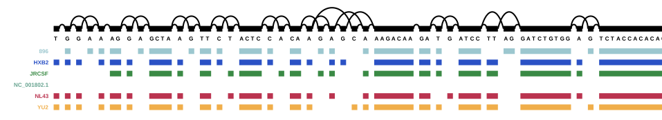
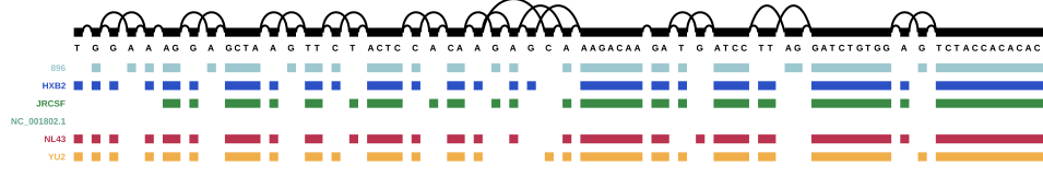
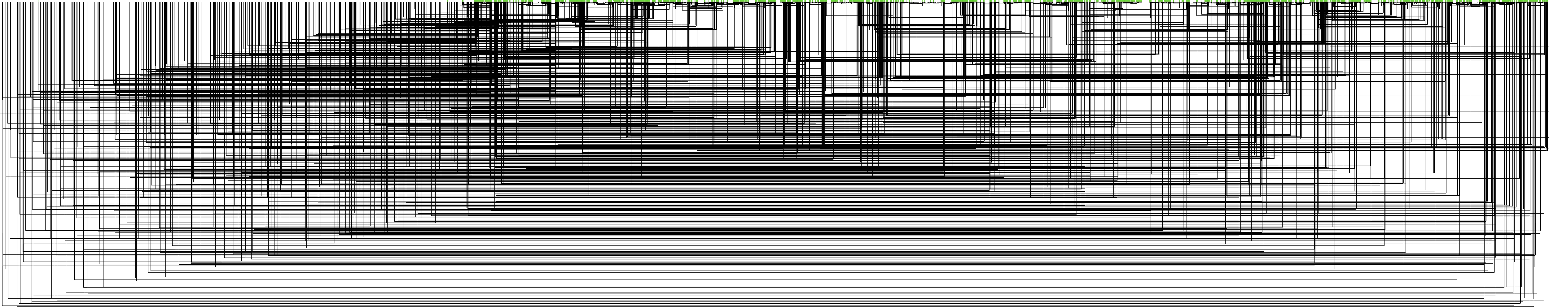
vg viz -x 6ref_annot.xg -o pics/6ref_annot.svg
Variant graph with annotation - start
This worked, yay!
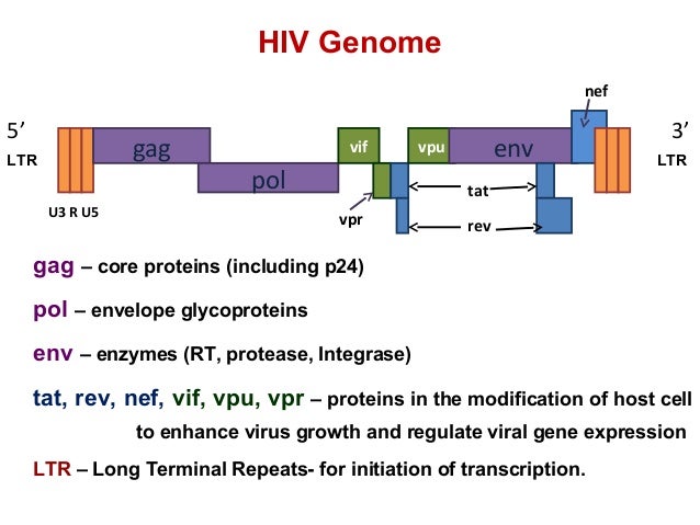
As a reminder: 896, HXB2, JRCSF, NL43, and YU2 are the five reference genomes from the mix, and NC_00.1802.1 is the HIV-1 reference genome I downloaded from NCBI. The other paths that are now present in the graph are the genes from the annotation. Scroll back up to the HIV genome structure figure for a reminder of the HIV genome structure.
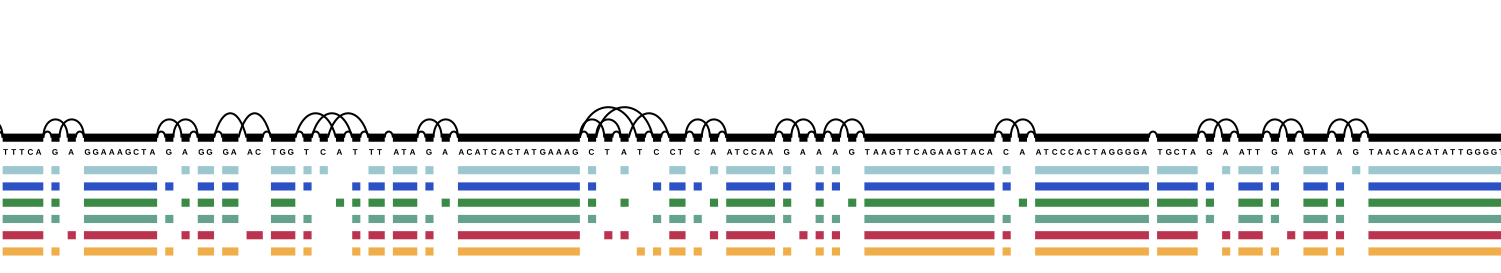
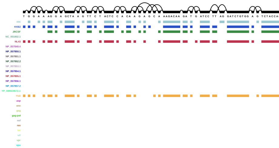
Variant graph with annotation - first genes
It seems that four entries in the annotation are the same in the beginning - NP_057849.4, NP_057850.1, gag, and gag-pol, but NP_057849.4 and gag end sooner than the other two, so I assume that NP_057849.4 is, in fact, gag, and NP_057850.1 is gag-pol (i.e. the gag gene together with the pol gene).
A similar pattern can be seen throughout the rest of the annotated graph - there is always one gene name and one associated “NP number”: in the annotation, “gene” features are the ones with the gene names, and “CDS” features are the ones with the NP numbers. Apparently vg annotate adds both of those features (while ignoring others like untranslated regions and “biological regions”). This is a little annoying and I think for real projects, annotations will probably have to be cleaned, as long as it’s not possible to select which features vg annotate will use.
One simple way to analyse sequence variability now is to count the number of nodes per annotated gene - more nodes should mean more variable sequences when you normalise for the gene length.
This analysis should be easy to do in R using the graph in JSON format:
vg view 6ref_annot.vg -j > 6ref_annot.json
graph path '' invalid: edge from 3116 end to 3171 start does not exist
graph path '' invalid: edge from 246 end to 3174 start does not exist
graph path '' invalid: edge from 3174 end to 3179 start does not exist
graph path '' invalid: edge from 3148 end to 3151 start does not exist
[vg view] warning: graph is invalid!
The conversion seems to have worked despite the error messages, so I wrote an R script that uses tidyjson and the tidyverse to clean up the graph and plot the number of nodes per gene (normalised by gene length).
Since the GFF annotation file is a little “crowded” with information and not easily readable by R, I downloaded the tabular version of the HIV-1 annotation for this task. Another step I took to make this analysis a little easier was extracting just the paths from the graph into JSON format, since the whole graph proved hard to parse:
jq '.path' 6ref_annot.json > 6ref_annot_paths.json
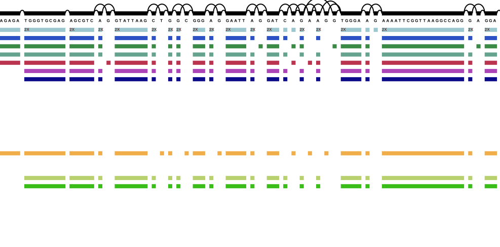
At first I used the “Length” information from the tabular annotation file to normalise the number of nodes per gene, which lead to this figure:
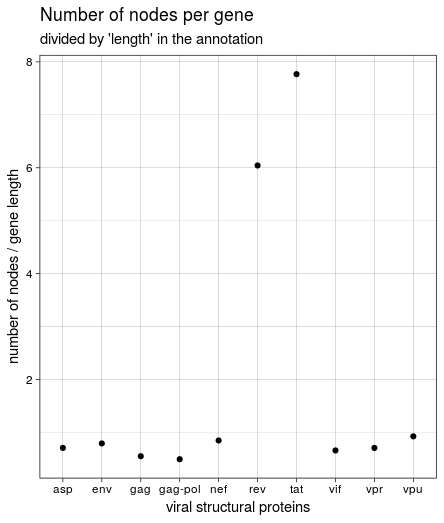
This was not the same result we got in the course, though, and it seemed weird that rev and tat had such a high number of nodes while being very short. Looking back at the HIV genome structure again shows why: both genes seem to encompass vpu and (partly) env. The length listed in the annotation is very short and relates to the protein; the region covered between “start” and “end” of all genes is much larger. Since the start and end values were used to create the paths through the graph, I used these values to calculate gene length and create the figure again:
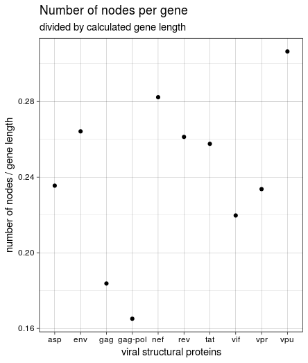
This is the same result we got in the course: the most variable genes in the HIV(-1) genome based on the number of nodes in the graph are vpu, nef, and env. vpu and env are expressed from a bicistronic mRNA, with Env being one of the viral structural proteins while Vpu is specific for HIV-1 and therefore an accessory regulatory protein. Nef is “the most immunogenic of the accessory proteins” of HIV, as it is one of the first produced proteins in infected cells.
By far the least variable gene(s) are gag an pol, or gag-pol. They express core structural proteins as a polyprotein and probably have to be more conserved.
Open questions
- How to decide on a
-xsetting in minimap2? - What is the significance of the additional output of
odgi viz? - Is there still a pileup option/tool somewhere, if
vg augmentdoesn’t do it? - What is the problem with
vg augment -ifor mapped reads? - What’s so tricky about augmenting the graph with long reads? Why don’t they fit to the references?