Day 1 - Toy Examples
Table of Contents
I want to work through the exercises we did at CPANG19, because I didn’t have a chance to try everything that’s possible and there are some things I think I should know before I start with my own examples. The guide in the vg Wiki is probably also useful, but we learned it’s a little outdated.
Let’s start with Day 1.
Getting started
I’m not going to git clone vg again like the instructions say, I’ve put enough work into that already, and I do have the test/ directory where I expect it to be, so I’ll just create a directory to work in and a symbolic link to the test data.
cd /data3/genome_graphs/CPANG/static/playground
mkdir day1
cd day1
ln -s ../../../vg/test/tiny
Constructing and viewing graphs
Graph construction
Constructing a graph from a single sequence fasta file is easy, even though the path to vg is a bit annoying to use:
/data3/genome_graphs/vg/bin/vg construct -r tiny/tiny.fa -m 32 > tiny.ref.vg
Maybe I can symlink the vg executable to /usr/bin/ and then use it without the full path.
cd /usr/bin/
sudo ln -s /data3/genome_graphs/vg/bin/vg
cd /data3/genome_graphs/CPANG/playground/day1/
vg construct
usage: vg construct [options] >new.vg
options:
construct from a reference and variant calls:
    -r, --reference FILE   input FASTA reference (may repeat)
    -v, --vcf FILE         input VCF (may repeat)
    -n, --rename V=F       rename contig V in the VCFs to contig F in the FASTAs (may repeat)
    -a, --alt-paths        save paths for alts of variants by variant ID
    -R, --region REGION    specify a particular chromosome or 1-based inclusive region
    -C, --region-is-chrom  don't attempt to parse the region (use when the reference
                           sequence name could be inadvertently parsed as a region)
    -z, --region-size N    variants per region to parallelize (default: 1024)
    -t, --threads N        use N threads to construct graph (defaults to numCPUs)
    -S, --handle-sv        include structural variants in construction of graph.
    -I, --insertions FILE  a FASTA file containing insertion sequences
                           (referred to in VCF) to add to graph.
    -f, --flat-alts N      don't chop up alternate alleles from input VCF
    -i, --no-trim-indels   don't remove the 1bp reference base from alt alleles of indels.
construct from a multiple sequence alignment:
    -M, --msa FILE         input multiple sequence alignment
    -F, --msa-format       format of the MSA file (options: fasta, clustal; default fasta)
    -d, --drop-msa-paths   don't add paths for the MSA sequences into the graph
shared construction options:
    -m, --node-max N       limit the maximum allowable node sequence size (defaults to 32)
                           nodes greater than this threshold will be divided
                           Note: nodes larger than ~1024 bp can't be GCSA2-indexed
    -p, --progress         show progress
Perfect!
Great, so I did vg construct -r tiny/tiny.fa -m 32 > tiny.ref.vg. The fasta reference was marked with the -r, and the -m meant I restricted the node size to 32 nucleotides, which is the standard. This means I should now have a linear graph in the form of multiple connected 32 bp nodes. Let’s see if that’s true.
Graph visualisation
vg view tiny.ref.vg
This command returns a graph in GFA format:
H       VN:Z:1.0
S       1       CAAATAAGGCTTGGAAATTTTCTGGAGTTCTA
S       2       TTATATTCCAACTCTCTG
P       x       1+,2+   32M,18M
L       1       +       2       +       0M
The “H” marks the header, the “S” stands for segment, so we have two segments/nodes, “P” is the path through the nodes, and the “L” is the link actually connecting the segments. There can sometimes also be a “C”, denoting the containment of one segment in another.
JSON
vg view -j tiny.ref.vg | jq
The -j option creates the graph in JSON format, which can be nicely viewed using jq:
{
  "edge": [
    {
      "from": "1",
      "to": "2"
    }
  ],
  "node": [
    {
      "id": "1",
      "sequence": "CAAATAAGGCTTGGAAATTTTCTGGAGTTCTA"
    },
    {
      "id": "2",
      "sequence": "TTATATTCCAACTCTCTG"
    }
  ],
  "path": [
    {
      "mapping": [
        {
          "edit": [
            {
              "from_length": 32,
              "to_length": 32
            }
          ],
          "position": {
            "node_id": "1"
          },
          "rank": "1"
        },
        {
          "edit": [
            {
              "from_length": 18,
              "to_length": 18
            }
          ],
          "position": {
            "node_id": "2"
          },
          "rank": "2"
        }
      ],
      "name": "x"
    }
  ]
}
jq can also be used to filter the output:
vg view -j tiny.ref.vg | jq '.node[].sequence'
"CAAATAAGGCTTGGAAATTTTCTGGAGTTCTA"
"TTATATTCCAACTCTCTG"
DOT
The DOT output generated with the -d option can be redirected to graphviz to create a PDF file of the graph:
vg view -d tiny.ref.vg | dot -Tpdf -o tiny.ref.pdf
DOT version of tiny reference graph
This linear graph is pretty boring and no better than a regular reference sequence. Luckily, we have a VCF (variant call format) file with variants that can be included in the graph. That is also done using vg construct, adding the -v option to mark the VCF input file:
Adding variants to the graph
vg construct -r tiny/tiny.fa -v tiny/tiny.vcf.gz -m 32 > tiny.vg
vg view -d tiny.vg | dot -Tpdf -o tiny.pdf
It is also possible to show the original reference path in the DOT output by adding the -p option to the vg view call:
vg view -dp tiny.vg | dot -Tpdf -o tiny_path.pdf
DOT version of tiny graph with path
This adds a path (usually with funny symbols) to the graph and at every edge notes the node that the path takes in order to be the reference sequence.
The -S argument (--simple-dot) simplifies the DOT output by removing node labels/sequences:
vg view -dpS tiny.vg | dot -Tpdf -o tiny_simple.pdf
simplifed DOT version of tiny graph with path
For a different visual layout of the graph, use Neato, which is part of the graphviz package:
vg view -dpS tiny.vg | neato -Tpdf -o tiny_neato.pdf
simplifed DOT version of tiny graph with path in Neato
Note that Neato works best with the simplified version of the graph, as it doesn’t display longer sequences well.
Since vg view so easily converts between different formats, it’s also quite easy to manipulate the graph itself. The example included here removes the path from the GFA graph using grep -v (which only finds non-matching lines) and then visualises it again:
vg view tiny.vg > tiny.gfa
cat tiny.gfa | grep -v ^P | vg view -dp - | dot -Tpdf -o tiny.no_path.pdf
Or maybe not:
terminate called after throwing an instance of 'std::runtime_error'
  what():  [io::ProtobufIterator] could not parse message
ERROR: Signal 6 occurred. VG has crashed. Run 'vg bugs --new' to report a bug.
Stack trace path: /tmp/vg_crash_ZtE85h/stacktrace.txt
vg view has the -F option to make it clear that the input is in GFA format, and the -p option doesn’t make sense if you don’t have paths to display:
cat tiny.gfa | grep -v ^P | vg view -dF - | dot -Tpdf -o tiny.no_path.pdf
simplifed DOT version of tiny graph with no path
As output, this doesn’t have any advantage over just not adding the path in the vg view call with -p, but in other settings it might be helpful to be able to edit the graph itself, e.g. for looking for specific regions.
Mapping reads to a graph
Graph construction
We are using a bigger example to map reads to now, 1 Mbp of the 1000 Genomes data for a certain region of chromosome 20:
ln -s ../../../vg/test/1mb1kgp
First, we need to create the reference graph from a linear fasta sequence and the known sequence variation:
vg construct -r 1mb1kgp/z.fa -v 1mb1kgp/z.vcf.gz > z.vg
The command results in a few warnings about unsupported variant alleles:
warning:[vg::Constructor] Unsupported variant allele "<CN0>"; Skipping variant(s) z     13790   BI_GS_DEL1_B1_P2734_15  T <CN0>    100     PASS    AC=1;AF=0.000199681;AFR_AF=0;AMR_AF=0;AN=5008;CIEND=-75,76;CIPOS=-75,76;CS=DEL_union;DP=15541;EAS_AF=0;END=1017354;EUR_AF=0.001;NS=2504;SAS_AF=0;SVLEN=-3562;SVTYPE=DEL !
warning:[vg::Constructor] Unsupported variant allele "<INS:ME:ALU>"; Skipping variant(s) z      14169   ALU_umary_ALU_12010G       <INS:ME:ALU>    100     PASS    AC=43;AF=0.00858626;AFR_AF=0.0303;AMR_AF=0.0043;AN=5008;CS=ALU_umary;DP=18053;EAS_AF=0;EUR_AF=0;MEINFO=AluUndef,2,281,+;NS=2504;SAS_AF=0;SVLEN=279;SVTYPE=ALU;TSD=null !
warning:[vg::Constructor] Unsupported variant allele "<CN2>"; Skipping variant(s) z     490168  DUP_gs_CNV_20_1490168_1549769      G       <CN2>   100     PASS    AC=1;AF=0.000199681;AFR_AF=0;AMR_AF=0;AN=5008;CS=DUP_gs;DP=21874;EAS_AF=0;END=1549769;EUR_AF=0;NS=2504;SAS_AF=0.001;SVTYPE=DUP !
I can’t remember if we’ve seen this in the course, but since it only skips those variants, I’ll ignore this for now.
Graph in Bandage
The course instructions already warn here that this 1 Mbp graph is too big to be viewed with the methods introduced so far, so I’ll have a quick look in Bandage instead, which I have already running on my PC. Bandage can visualise graphs in GFA format:
vg view z.vg > z.gfa
The graph consist of 102,996 nodes, and - in the zoomed out view in Bandage - still looks pretty linear. There are most likely no major structural variants included, but a lot of single nucleotide polymorphisms (SNPs) and insertions or deletions (indels).
z.gfa detail in Bandage
Graph indexing
In order to finally map reads to the graph, I have to index it in two different ways: vg needs an XG index (a succinct representation) and a GCSA index (k-mer based).
vg index -x z.xg -g z.gcsa -k 16 z.vg
The indexing already takes some time, which I remember is mostly due to the GCSA index. The -k option is only needed for GCSA, as it gives the program the length of the k-mers to use. How to choose this was not really discussed in the course, but it can influence sensitivity and run time of the read mapping.
Extracting and visualising a subgraph by node ID
A nice advantage of indexing the graph is that we can now also extract subgraphs using vg find and the ID of a node of interest:
vg find -n 2401 -x z.xg -c 10 | vg view -dp - | dot -Tpdf -o 2401c10.pdf
The -c option is for “context”", so how many nodes should be included around the one of interest:
Read simulation and mapping
Since no reads for mapping were included in this example dataset, they have to be simulated from the existing graph with included variants. vg sim takes the XG index of a graph (-x), the length (-l) and number (-n) of the reads to simulate, and the base substitution rate (-e) and indel rate (-i). It can put out raw sequences or sequences with their true alignments in binary GAM (Graph Alignment Map) format, which is useful to later test how successful the mapping was (when using the graph from which the reads were simulated).
vg sim -x z.xg -l 100 -n 1000 -e 0.01 -i 0.005 -a > z.sim
Mapping can be done with FASTA or FASTQ sequences, but also with the GAM format that was the output of the read simulation. The output will also again be in GAM format.
vg map -x z.xg -g z.gcsa -G z.sim > z.gam
Visualising read alignment
Read alignments can be visualised with vg view, but of course it’s again not possible to see all at once. Instead, we can look at the first alignment using a combination of commands: vg view with the -a argument can read the GAM format, from which we then extract the first line (i.e. the first alignment) and convert that into its own GAM (-G) file (I assume that the -a here tells vg view that the JSON (-J) input is of a GAM file). vg find can then find regions in the indexed graph touched by this alignment, vg view creates a DOT format output (-d) of the GAM with the alignment (-A), and that is visualised with graphviz as usual. (And that is why I need these course materials in order to be able to use vg to its full potential.)
vg view -a z.gam | head -1 | vg view -JaG - > first_aln.gam
vg find -x z.xg -G first_aln.gam | vg view -dA first_aln.gam - | dot -Tpdf -o first_aln.pdf
DOT version of subgraph with first alignment
The output shows blue and yellow annotations above the subgraph, denoting the mapping of the read. Blue means it’s an exact match, yellow marks a mismatch. The graph shows the mapping quality (60) and identity (0.99) of the read compared to the graph, as well as the read name (above the numbers), and the score (97) at the first mapped position to the right of the subgraph. It then shows the mappings to a path, including the position with node ID and forward/reverse information, as well as a “from” and a “to” length which I cannot explain. I think the rank basically gives the order in which the fragments map - reading from right to left in this case.
The next two alignments are not reversed, I’ll check what happens if I include them here. It might not be possible, since they mapped to very different nodes.
vg view -a z.gam | head -3 | vg view -JaG - > first3_aln.gam
vg find -x z.xg -G first3_aln.gam | vg view -dA first3_aln.gam - | dot -Tpdf -o first3_aln.pdf
DOT version of subgraphs with first three alignments
Cool! As I hoped, I now have three subgraphs in my PDF file.
They seem to be sorted in reverse order by node ID (highest number on top). The two reads that mapped on the forward “strand” have their additional information listed in the beginning: names, scores, quality, and identity. The “length” numbers are also the same here for “to” and “from”, and while I’m not sure why they are called that, I think they really do mean the length of the node sequence to which the read maps (or the length of the read mapping to the node?). The offset tells where the mapping starts, and then the lengths are usually to the end of the node, but not all mappings have an offset. When there are mismatches, the length that matches is given, then length and sequence of the mismatch, then again the length of the match.
The format is quite complicated, maybe I’ll get deeper into that later…
It’s also possible to again create a simplified graph with graphviz, maybe that’s less confusing.
vg find -x z.xg -G first3_aln.gam | vg view -dSA first3_aln.gam - | dot -Tpdf -o first3_aln_simple.pdf
simplified DOT version of subgraphs with first three alignments
Much simpler indeed! The mismatches are better hidden now, though - the colour code is ranged from green to red based on the mapping quality, so single nucleotide mismatches are not visible, in this example at least.
Comparison of mapping and true read location
To really evaluate the mapping success, the read alignments can be compared to the true paths saved in the GAM file with the simulated reads. This is again done with vg map using the --compare option (-j leads to output in JSON format):
vg map -x z.xg -g z.gcsa -G z.sim --compare -j > z_comp.json
The JSON output contains information about how correct the mapping was:
jq .correct z_comp.json
We can quickly calculate the mean correctness using awk:
jq .correct z_comp.json | awk '{i+=$1; n+=1} END {print i/n}'
0.99529
This is a good tool to test different mapping parameters - we can test how they influence the correctness of the mapping. In the course example, we used a high minimum match length:
vg map -k 51 -x z.xg -g z.gcsa -G z.sim --compare -j | jq .correct | sed s/null/0/ | awk '{i+=$1; n+=1} END {print i/n}'
The additional sed command replaces “null” with the number 0 since that would break the calculation. The resulting mean correctness with the high minimum match length is:
0.82213
because we’re throwing away information we need for a correct mapping with this restriction. The reads are only 100 bp long - requiring a perfect match over at least half of one is very optimistic.
Exploring the benefits of graphs for read mapping
In order to analyse how a genome graph with sequence variation can improve the mapping of sequencing reads, we generated reference graphs with different numbers of variants - filtering by allele frequency. This is done using vcffilter from the vcflib package authored by Erik, which is available via bioconda, yay!
sudo -i
conda install -c conda-forge -c bioconda -c defaults vcflib
exit
Filtering with a minimum allele frequency should remove rare variants from the VCF and - in turn - from the reference graph, but I also want to set filter for a maximum frequency for comparison, to see what happens when only rare variants are included in the graph. I’ll try writing a little bash script to filter the original VCF file by allele frequency…
touch filter_vcf_minAF.sh
chmod +x filter_vcf_minAF.sh
./filter_vcf_minAF.sh
0.7
warning:[vg::Constructor] Unsupported variant allele "<CN0>"; Skipping variant(s) z     560739  YL_CN_CHB_4219  T       <CN0>      100     PASS    AC=4099;AF=0.81849;AFR_AF=0.9213;AMR_AF=0.6527;AN=5008;CIEND=-500,1000;CIPOS=-1000,500;CS=DEL_union;DP=20713;EAS_AF=0.7867;END=1593685;EUR_AF=0.7903;NS=2504;SAS_AF=0.8589;SVLEN=-32947;SVTYPE=DEL !
0.97147
0.5
warning:[vg::Constructor] Unsupported variant allele "<CN0>"; Skipping variant(s) z     389096  UW_VH_3735      G       <CN0>      100     PASS    AC=2647;AF=0.528554;AFR_AF=0.2685;AMR_AF=0.5922;AN=5008;CIEND=0,478;CIPOS=-443,0;CS=DEL_union;DP=18400;EAS_AF=0.7996;END=1390815;EUR_AF=0.5;NS=2504;SAS_AF=0.5849;SVLEN=2051;SVTYPE=DEL !
0.97188
0.1
warning:[vg::Constructor] Unsupported variant allele "<CN0>"; Skipping variant(s) z     389096  UW_VH_3735      G       <CN0>      100     PASS    AC=2647;AF=0.528554;AFR_AF=0.2685;AMR_AF=0.5922;AN=5008;CIEND=0,478;CIPOS=-443,0;CS=DEL_union;DP=18400;EAS_AF=0.7996;END=1390815;EUR_AF=0.5;NS=2504;SAS_AF=0.5849;SVLEN=2051;SVTYPE=DEL !
warning:[vg::Constructor] Unsupported variant allele "<INS:ME:ALU>"; Skipping variant(s) z      546228  ALU_umary_ALU_12014G       <INS:ME:ALU>    100     PASS    AC=2031;AF=0.405551;AFR_AF=0.4637;AMR_AF=0.2882;AN=5008;CS=ALU_umary;DP=17504;EAS_AF=0.5615;EUR_AF=0.2475;MEINFO=AluUndef,1,281,+;NS=2504;SAS_AF=0.4121;SVLEN=280;SVTYPE=ALU;TSD=AAGAAATGTTTCCTG !
0.97275
0.01
warning:[vg::Constructor] Unsupported variant allele "<INS:ME:ALU>"; Skipping variant(s) z      90955   ALU_umary_ALU_12011A       <INS:ME:ALU>    100     PASS    AC=58;AF=0.0115815;AFR_AF=0.0424;AMR_AF=0.0029;AN=5008;CS=ALU_umary;DP=19023;EAS_AF=0;EUR_AF=0;MEINFO=AluYa5,4,281,+;NS=2504;SAS_AF=0;SVLEN=277;SVTYPE=ALU;TSD=AGAGAGGCA !
warning:[vg::Constructor] Unsupported variant allele "<CN0>"; Skipping variant(s) z     389096  UW_VH_3735      G       <CN0>      100     PASS    AC=2647;AF=0.528554;AFR_AF=0.2685;AMR_AF=0.5922;AN=5008;CIEND=0,478;CIPOS=-443,0;CS=DEL_union;DP=18400;EAS_AF=0.7996;END=1390815;EUR_AF=0.5;NS=2504;SAS_AF=0.5849;SVLEN=2051;SVTYPE=DEL !
0.97434
This script does the following:
- filter the given VCF file with a minimum allele frequency (AF > 0.7, 0.5, 0.1, 0.01), which is printed to the console
- construct a genome graph using the filtered VCF file
- index the genome graph
- map the previously simulated reads to the graph
- calculate the mean identity of the reads and print that to the console
There are again some warnings about unsupported variants. Ignoring those, we get the following data:
| AF threshold | mean identity | xg file size |
|---|---|---|
| 0.7 | 0.97147 | 3.0M |
| 0.5 | 0.97188 | 3.1M |
| 0.1 | 0.97275 | 3.4M |
| 0.01 | 0.97434 | 4.0M |
The lower the threshold, the better is the read identity and the bigger is the index file (as well as the graph itself), as more variants are included.
What happens when I do the same, but with a maximum allele frequency filter?
touch filter_vcf_maxAF.sh
chmod +x filter_vcf_maxAF.sh
./filter_vcf_maxAF.sh
0.7
warning:[vg::Constructor] Unsupported variant allele "<CN0>"; Skipping variant(s) z     13790   BI_GS_DEL1_B1_P2734_15  T <CN0>    100     PASS    AC=1;AF=0.000199681;AFR_AF=0;AMR_AF=0;AN=5008;CIEND=-75,76;CIPOS=-75,76;CS=DEL_union;DP=15541;EAS_AF=0;END=1017354;EUR_AF=0.001;NS=2504;SAS_AF=0;SVLEN=-3562;SVTYPE=DEL !
warning:[vg::Constructor] Unsupported variant allele "<INS:ME:ALU>"; Skipping variant(s) z      14169   ALU_umary_ALU_12010G       <INS:ME:ALU>    100     PASS    AC=43;AF=0.00858626;AFR_AF=0.0303;AMR_AF=0.0043;AN=5008;CS=ALU_umary;DP=18053;EAS_AF=0;EUR_AF=0;MEINFO=AluUndef,2,281,+;NS=2504;SAS_AF=0;SVLEN=279;SVTYPE=ALU;TSD=null !
warning:[vg::Constructor] Unsupported variant allele "<CN2>"; Skipping variant(s) z     490168  DUP_gs_CNV_20_1490168_1549769      G       <CN2>   100     PASS    AC=1;AF=0.000199681;AFR_AF=0;AMR_AF=0;AN=5008;CS=DUP_gs;DP=21874;EAS_AF=0;END=1549769;EUR_AF=0;NS=2504;SAS_AF=0.001;SVTYPE=DUP !
0.98679
0.5
warning:[vg::Constructor] Unsupported variant allele "<CN0>"; Skipping variant(s) z     13790   BI_GS_DEL1_B1_P2734_15  T <CN0>    100     PASS    AC=1;AF=0.000199681;AFR_AF=0;AMR_AF=0;AN=5008;CIEND=-75,76;CIPOS=-75,76;CS=DEL_union;DP=15541;EAS_AF=0;END=1017354;EUR_AF=0.001;NS=2504;SAS_AF=0;SVLEN=-3562;SVTYPE=DEL !
warning:[vg::Constructor] Unsupported variant allele "<INS:ME:ALU>"; Skipping variant(s) z      14169   ALU_umary_ALU_12010G       <INS:ME:ALU>    100     PASS    AC=43;AF=0.00858626;AFR_AF=0.0303;AMR_AF=0.0043;AN=5008;CS=ALU_umary;DP=18053;EAS_AF=0;EUR_AF=0;MEINFO=AluUndef,2,281,+;NS=2504;SAS_AF=0;SVLEN=279;SVTYPE=ALU;TSD=null !
warning:[vg::Constructor] Unsupported variant allele "<CN2>"; Skipping variant(s) z     490168  DUP_gs_CNV_20_1490168_1549769      G       <CN2>   100     PASS    AC=1;AF=0.000199681;AFR_AF=0;AMR_AF=0;AN=5008;CS=DUP_gs;DP=21874;EAS_AF=0;END=1549769;EUR_AF=0;NS=2504;SAS_AF=0.001;SVTYPE=DUP !
0.98647
0.1
warning:[vg::Constructor] Unsupported variant allele "<CN0>"; Skipping variant(s) z     13790   BI_GS_DEL1_B1_P2734_15  T <CN0>    100     PASS    AC=1;AF=0.000199681;AFR_AF=0;AMR_AF=0;AN=5008;CIEND=-75,76;CIPOS=-75,76;CS=DEL_union;DP=15541;EAS_AF=0;END=1017354;EUR_AF=0.001;NS=2504;SAS_AF=0;SVLEN=-3562;SVTYPE=DEL !
warning:[vg::Constructor] Unsupported variant allele "<INS:ME:ALU>"; Skipping variant(s) z      14169   ALU_umary_ALU_12010G       <INS:ME:ALU>    100     PASS    AC=43;AF=0.00858626;AFR_AF=0.0303;AMR_AF=0.0043;AN=5008;CS=ALU_umary;DP=18053;EAS_AF=0;EUR_AF=0;MEINFO=AluUndef,2,281,+;NS=2504;SAS_AF=0;SVLEN=279;SVTYPE=ALU;TSD=null !
warning:[vg::Constructor] Unsupported variant allele "<CN2>"; Skipping variant(s) z     490168  DUP_gs_CNV_20_1490168_1549769      G       <CN2>   100     PASS    AC=1;AF=0.000199681;AFR_AF=0;AMR_AF=0;AN=5008;CS=DUP_gs;DP=21874;EAS_AF=0;END=1549769;EUR_AF=0;NS=2504;SAS_AF=0.001;SVTYPE=DUP !
0.98561
0.01
warning:[vg::Constructor] Unsupported variant allele "<CN0>"; Skipping variant(s) z     13790   BI_GS_DEL1_B1_P2734_15  T <CN0>    100     PASS    AC=1;AF=0.000199681;AFR_AF=0;AMR_AF=0;AN=5008;CIEND=-75,76;CIPOS=-75,76;CS=DEL_union;DP=15541;EAS_AF=0;END=1017354;EUR_AF=0.001;NS=2504;SAS_AF=0;SVLEN=-3562;SVTYPE=DEL !
warning:[vg::Constructor] Unsupported variant allele "<INS:ME:ALU>"; Skipping variant(s) z      14169   ALU_umary_ALU_12010G       <INS:ME:ALU>    100     PASS    AC=43;AF=0.00858626;AFR_AF=0.0303;AMR_AF=0.0043;AN=5008;CS=ALU_umary;DP=18053;EAS_AF=0;EUR_AF=0;MEINFO=AluUndef,2,281,+;NS=2504;SAS_AF=0;SVLEN=279;SVTYPE=ALU;TSD=null !
warning:[vg::Constructor] Unsupported variant allele "<CN2>"; Skipping variant(s) z     490168  DUP_gs_CNV_20_1490168_1549769      G       <CN2>   100     PASS    AC=1;AF=0.000199681;AFR_AF=0;AMR_AF=0;AN=5008;CS=DUP_gs;DP=21874;EAS_AF=0;END=1549769;EUR_AF=0;NS=2504;SAS_AF=0.001;SVTYPE=DUP !
0.98413
| AF threshold | mean identity | xg file size |
|---|---|---|
| 0.7 | 0.98679 | 9.4M |
| 0.5 | 0.98647 | 9.3M |
| 0.1 | 0.98561 | 9.0M |
| 0.01 | 0.98413 | 8.4M |
Apparently, rare alleles are more frequent in the VCF file than common ones - setting a maximum limit to the allele frequency leads to bigger files and a higher mean identity than setting a minimum limit. Other than that, the results look as expected: the higher the threshold, the more variants are included and the better is the mean identity.
Conclusion
Including variation in a genome graph used as reference for read mapping increases the read identity.
Mapping using real data to examine the improvement
The course also provided links to two sets of real sequencing reads for the example region used here: one that was part of the 1000 Genomes Project (NA12878), so these variants should be included already, and one that wasn’t (NA24385).
samtools view -b ftp://ftp-trace.ncbi.nlm.nih.gov/giab/ftp/data/NA12878/NIST_NA12878_HG001_HiSeq_300x/RMNISTHS_30xdownsample.bam 20:1000000-2000000 > NA12878.20_1M-2M.30x.bam
[E::bgzf_read] Read block operation failed with error 2 after 0 of 4 bytes
[main_samview] retrieval of region "20:1000000-2000000" failed due to truncated file or corrupt BAM index file
samtools view: error closing "ftp://ftp-trace.ncbi.nlm.nih.gov/giab/ftp/data/NA12878/NIST_NA12878_HG001_HiSeq_300x/RMNISTHS_30xdownsample.bam": -1
Hmm, now I have a file called “NA12878.20_1M-2M.30x.bam” and one called “RMNISTHS_30xdownsample.bam.bai”, and the .bam.bai index file is much larger than the BAM file. I assume the index is for the whole data set, while the BAM file should only comprise our region of interest.
I’ll try to check if the file is good to use despite the error.
samtools flagstat NA12878.20_1M-2M.30x.bam
0 + 0 in total (QC-passed reads + QC-failed reads)
0 + 0 secondary
0 + 0 supplementary
0 + 0 duplicates
0 + 0 mapped (N/A : N/A)
0 + 0 paired in sequencing
0 + 0 read1
0 + 0 read2
0 + 0 properly paired (N/A : N/A)
0 + 0 with itself and mate mapped
0 + 0 singletons (N/A : N/A)
0 + 0 with mate mapped to a different chr
0 + 0 with mate mapped to a different chr (mapQ>=5)
Apparently it isn’t, as there don’t seem to be any reads inside.
Maybe the other example will work better.
wget http://hypervolu.me/~erik/tmp/HG002-NA24385-20_1M-2M-50x.bam
--2019-10-09 13:02:11--  http://hypervolu.me/~erik/tmp/HG002-NA24385-20_1M-2M-50x.bam
Connecting to 172.16.20.248:3128... connected.
Proxy request sent, awaiting response... 200 OK
Length: 34389537 (33M)
Saving to: ‘HG002-NA24385-20_1M-2M-50x.bam’

HG002-NA24385-20_1M-2M-50x.bam 100%[===================================================>]  32.80M  1.36MB/s    in 27s

2019-10-09 13:02:39 (1.21 MB/s) - ‘HG002-NA24385-20_1M-2M-50x.bam’ saved [34389537/34389537]
samtools flagstat HG002-NA24385-20_1M-2M-50x.bam
319020 + 0 in total (QC-passed reads + QC-failed reads)
522 + 0 secondary
0 + 0 supplementary
3701 + 0 duplicates
317742 + 0 mapped (99.60% : N/A)
318498 + 0 paired in sequencing
159230 + 0 read1
159268 + 0 read2
314199 + 0 properly paired (98.65% : N/A)
315942 + 0 with itself and mate mapped
1278 + 0 singletons (0.40% : N/A)
1360 + 0 with mate mapped to a different chr
1157 + 0 with mate mapped to a different chr (mapQ>=5)
That’s more like it! I will remove the truncated file from the 1000 Genome Project and only work with the other one.
rm NA12878.20_1M-2M.30x.bam RMNISTHS_30xdownsample.bam.bai
To prepare for the mapping comparison, the .bam file can be converted to two .fastq files (the data comes from paired-end mapping). I also have to install Sambamba to work with the output of bwa mem, and create the indices that bwa needs for the mapping.
samtools fastq -1 HG002-NA24385-20_1M-2M-50x_1.fq.gz -2 HG002-NA24385-20_1M-2M-50x_2.fq.gz HG002-NA24385-20_1M-2M-50x.bam
sudo -i
conda install -c bioconda sambamba
exit
bwa index 1mb1kgp/z.fa
Now I can do the actual mapping and analysis.
bwa mem 1mb1kgp/z.fa HG002-NA24385-20_1M-2M-50x_1.fq.gz | sambamba view -S -f json /dev/stdin | jq -cr '[.qname, .tags.AS] | @tsv' > bwa_mem.scores.tsv
vg map --drop-full-l-bonus -d z -f HG002-NA24385-20_1M-2M-50x_1.fq.gz -j | jq -cr '[.name, .score] | @tsv' > vg_map.scores.tsv
The course materials provided these commands, which do the following:
- map the reads with
bwa memto the linear reference z.fa - use
sambamba viewon the SAM output (-S) ofbwa memand convert to JSON (-f json) - use
jqto generate compact (-c) raw (-r) string output of the read name (“qname”) and the alignment score (“tags.AS”) - summarise these results in TSV format and write that to a file
and
- map the reads with
vg mapwithout using the full length bonus (I think this is to generate scores similar to bwa), generating a JSON output - use
jqto generate compact (-c) raw (-r) string output of the read name (“name”) and the alignment score (“score”) - summarise these results in TSV format and write that to a file
I wrote a quick R script to check out the differences between the mapping approaches. The first thing I noticed was that bwa apparently mapped a few (76) reads to two different locations, because I have two score entries for them. vg did not do that, and since I didn’t want to decide which score to use I removed both of the duplicates from the data.
On the other hand, there were a few reads (five) which did not have a score assigned in the vg data for some reason.
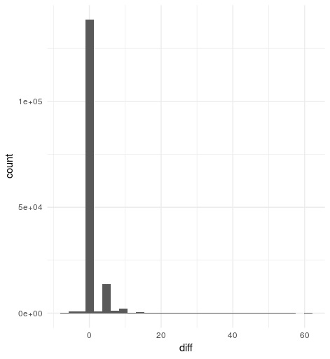
Histogram of score differences vg - bwa
Overall, it seems vg and bwa lead to very similar alignment scores - the difference between the two methods is zero in 136,615 of the cases (86%). There are 1,723 reads which mapped a little better with bwa than vg, but the biggest score difference is seven, and the most frequent one is four. Left are 20,813 (13%) reads that mapped better to the genome graph, with a score difference of up to 61, while the most frequent one is five.
Conclusion
In most cases, vg is equivalent to or better than bwa when using a genome graph with known variants included. The few cases where bwa was better than vg only showed small differences in the scores, which could also be due to slight differences in score calculation.
Cleaning up the directory
I think it’s a good idea to sort all the files in this directory by “project”:
mkdir construct_tiny
mkdir sim_reads
mkdir allele_frequency
mkdir real_data
mv tiny* construct_tiny/
mv 1mb1kgp 2401c10.pdf first* z* sim_reads/
mv *af* filter* allele_frequency/
mv HG* bwa* vg_map.scores.tsv real_data/
Although, maybe it would be easier to keep the images where they were…
mv construct_tiny/*.pdf .
mv sim_reads/*.pdf sim_reads/*.PNG .
mv real_data/bwa_vg_hist.png .
Note that to replicate the steps in this document, these new directories have to be used.
Open questions
- How to choose k for GCSA indexing or graph construction?
- What are the length values in the mapping results?
- Why do some reads not have a mapping score in vg?